****************nano vna user guide****************

NanoVNA User Guide

Introduction

This document is an unofficial user guide for NanoVNA. The URL is https://cho45.github.io/NanoVNA-manual/

Maintained on the github repository .

Please send a Pull-request if you have any changes, such as a conflict with the latest firmware.

It is also available in PDF format on the GitHub Releases page.

https://github.com/cho45/NanoVNA-manual/releases

What is NanoVNA

There are several types of hardware for NanoVNA, and this document covers the following hardware:

ttrftech version (original) ttrftech / NanoVNA
hugen79 version hugen79 / NanoVNA-H

These hardware have similar components on the circuit and common firmware is available.

What you need to work

At a minimum, you need:

NanoVNA body
SMA LOAD 50Ω
SMA SHORT
SMA OPEN
SMA Female to Female Through Connector
SMA Male to Male cable × 2

NanoVNA Basics

VNA (Vector Network Analyzer) measures the frequency characteristics of reflected power and transmitted power of a radio frequency network (RF Network).

NanoVNA measures the following factors:

Input voltage I / Q signal
I / Q signal of reflected voltage
I / Q signal of passing voltage

From this we calculate:

Reflection coefficients S11
Transmission coefficient S21

The following items that can be calculated from these can be displayed.

Return loss
Passage loss
Complex impedance
- resistance
- reactance
SWR

Such.

Oscillation frequency of NanoVNA

The NanoVNA measures the reflection coefficient and transmission coefficient for 101 points in the frequency band to be measured.

The local frequency of NanoVNA is from 50kHz to 300MHz. Higher frequencies use harmonic mode. The fundamental wave is not attenuated even in the harmonic mode. The usage modes for each frequency are as follows.

Up to 300 MHz: fundamental wave
300MHz to 900MHz: 3rd harmonic
900MHz to 1500MHz: 5th harmonic

Especially when checking the gain of the amplifier, it is necessary to pay attention to the fact that there is always a fundamental wave input.

The input is converted to an intermediate frequency of 5 kHz in each case. The signal is converted from analog to digital at 48kHz sampling. Digital data is processed by the MCU.

First thing to do

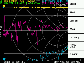
It must be calibrated first before it can be used. Initially, calibrate as follows.

Make sure START is 50kHz
Confirm that STOP is 900MHz
Perform calibration according to the calibration method

input method

The NanoVNA has the following inputs:

Tap and long tap on touch panel
Lever switch
- L / L Long press
- R / R Long press
- Press / Press and hold
Power slide switch

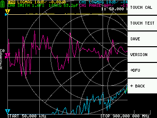
How to read the screen

Main screen

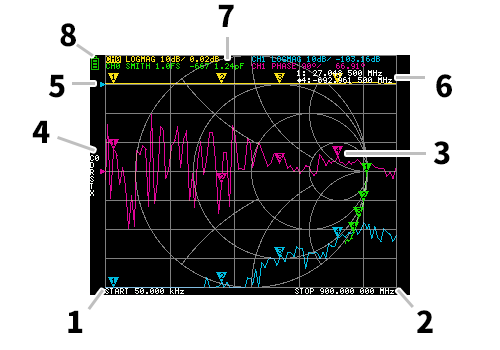
1. START 2. STOP frequency

Each frequency when the start / stop is specified is displayed.

3. Markers

The position of the marker for each trace is displayed. The selected marker can be moved in the following ways.

Drag marker on touch panel
Long press LR on lever switch

4. Calibration status

Displays the data number of the calibration being read and the error correction applied.

C0 C1 C2 C3 C4 : Indicates that the corresponding number of calibration data is loaded.
c0 c1 c2 c3 c4 : Each indicates that the corresponding number of calibration data has been loaded, but indicates that the frequency range has been changed after loading and interpolation is used for error correction.
D : Indicates that directivity error correction is applied
R : Indicates that refrection tracking error correction is applied
S : Indicates that source match error correction is applied
T : Indicates that transmission tracking error correction has been applied
X : Indicates that isolation (crosstalk) error correction has been applied

5. Reference position

Indicates the reference position of the corresponding trace. You can change the position with DISPLAY SCALE REFERENCE POSITION .

6. Marker status

The active marker you selected and one previously active marker are displayed.

7. Trace status

The status of each trace format and the value corresponding to the active marker are displayed.

For example, if the display is CH0 LOGMAG 10dB/ 0.02dB , read as follows.

Channel CH0 (reflection)
Format LOGMAG
Scale is 10dB
Current value is 0.02dB

The channel display of the active trace is inverted.

8. Battery status

If the battery is installed and D2 on the PCB is already mounted, the icon will be displayed according to the battery voltage.

Main screen 2

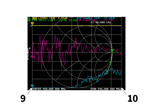
9. CENTER frequency 10. Span

The respective frequencies when the center frequency and span are specified are displayed.

Menu screen

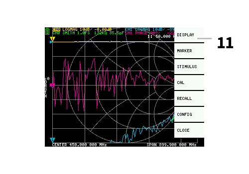
11. Menu

The menu can be displayed by the following operations.

When you tap anywhere other than the marker on the touch panel
Push the lever switch

Keypad screen

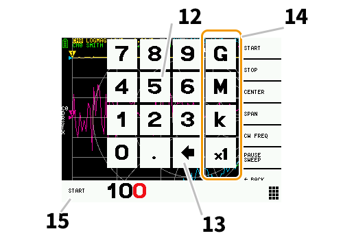
12. Numeric keys

Tap a number to enter one character.

13. Back key

Delete one character. If no characters have been entered, cancel the entry and return to the previous state.

14. Unit key

Multiplies the current input by the appropriate unit and terminates the input immediately. In the case of × 1, the entered value is set as it is.

15. Input field

The input target item name and the entered number are displayed.

Start measurement

Basic measurement sequence

Set the frequency range to measure
Perform calibration
Connect the DUT

Calibration method

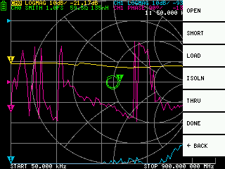
Calibration basically needs to be performed every time the frequency range to be measured is changed. If the error has been corrected correctly, the calibration status display on the screen will be Cn DRSTX . n is the data number being loaded.

However, NanoVNA can complement the existing calibration information and provide a somewhat correct display. This happens if you change the frequency range after loading the calibration data. At this time, the display of the calibration status on the screen is cn DRSTX . n is the data number being loaded.

Resets the current calibration status CAL RESET
Connect OPEN standard to CH0 port and execute CAL CALIBRATE OPEN .
Connect SHORT standard to CH0 port and execute CAL CALIBRATE SHORT .
Connect LOAD standard to CH0 port and execute CAL CALIBRATE LOAD .
Connect LOAD standard to CH0 and CH1 ports and execute CAL CALIBRATE ISOLN . If there is only one load, the CH0 port can be left unconnected.
Connect the cables to the CH0 and CH1 ports, connect the cables with through connectors, and execute CAL CALIBRATE THRU .
Finish calibration and calculate error correction information CAL CALIBRATE DONE
Specify the data number and save. CAL CALIBRATE SAVE SAVE 0

* It is necessary to import each calibration data after the display is sufficiently stable.

function

Trace display

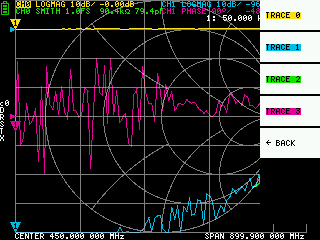
Up to four traces can be displayed, one of which is the active trace.

Traces show only what you need. To switch the display, select DISPLAY TRACE TRACE n .

There are the following ways to switch the active trace.

Tap the marker of the trace you want to activate
Select and display DISPLAY TRACE TRACE n . (If it is already displayed, you need to temporarily hide it)

Trace format

Each trace can have its own format. To change the format of the active trace DISPLAY FORMAT Select the format you want to change.

The display of each format is as follows.

LOGMAG : Logarithm of absolute value of measured value
PHASE : Phase from -180 ° to + 180 °
DELAY : Delay
SMITH : Smith chart
SWR : Standing Wave Ratio
POLAR : polar coordinate format
LINEAR : Absolute value of measured value
REAL : Real number of measured value
IMAG : Imaginary number of measured value
RESISTANCE : The resistance component of the measured impedance
REACTANCE : The reactance component of the measured impedance

Trace channel

The NanoVNA has two ports, CH0 CH1 . The following S parameters can be measured for each port.

CH0 S11 ( CH0 loss)
CH1 S21 (insertion loss)

To change the trace channel, select CH0 REFLECT or CH1 THROUGH of DISPLAY CHANNEL .

marker

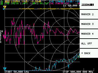
Up to four markers can be displayed. Markers are displayed from MARKER SELECT MARKER MARKER n . When you display a marker, the active marker is set to the displayed marker.

Time domain operation

The NanoVNA can simulate time domain measurements by processing the frequency domain data.

To convert measurement data to the time domain, select DISPLAY TRANSOFRM TRANSFORM ON . TRANSFORM ON is enabled, the measurement data is immediately converted to the time domain and displayed.

The following relationship exists between the time domain and the frequency domain.

Increasing the maximum frequency increases the time resolution
The shorter the measurement frequency interval (ie, the lower the maximum frequency), the longer the maximum time length

Therefore, there is a trade-off between the maximum time length and the time resolution.

To translate the length of time into distance, the following can be said.

If you want to increase the maximum measurement distance, you need to lower the maximum frequency
If you want to specify the distance accurately, you need to increase the maximum frequency.

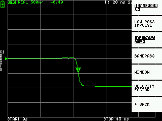
Time domain bandpass

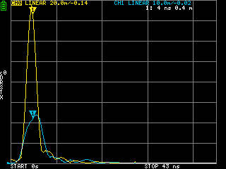
In bandpass mode, you can simulate the response of the DUT to an impulse signal.

The trace format can be set to LINEAR LOGMAG SWR .

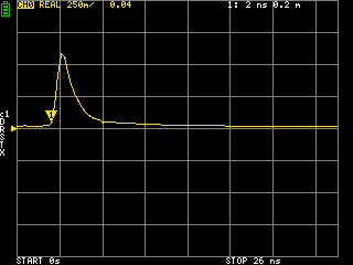
Below is an example of the impulse response of a bandpass filter.

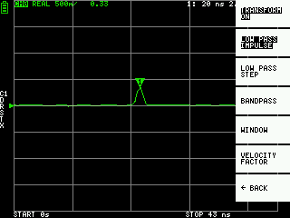
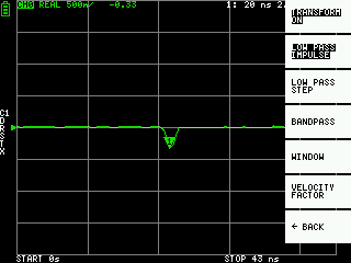
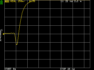
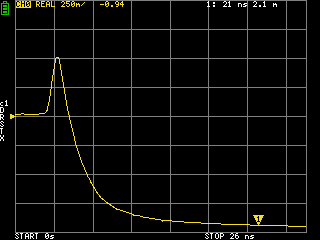
Time domain low pass impulse

In low-pass mode, you can simulate TDR. In low-pass mode, the start frequency must be set to 50kHz and the stop frequency must be set according to the distance to be measured.

Trace format can be set to REAL .

The following shows an example of the step response in the open state and the impulse response in the short state.

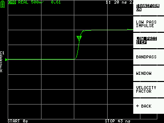
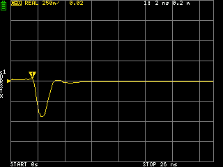
Time domain low pass step

In low-pass mode, you can simulate TDR. In low-pass mode, the start frequency must be set to 50kHz and the stop frequency must be set according to the distance to be measured.

Trace format can be set to REAL .

open:

short:

Step response example

Capacitive short:

Inductive short:

Discontinuous capacitive (C in parallel):

Inductive discontinuity (L in series):

Time domain window

The measurable range is a finite number, with a minimum frequency and a maximum frequency. Windows can be used to smooth out this discontinuous measurement data and reduce ringing.

There are three levels of windows.

MINIMUM (no window, ie same as rectangular window)
NORMAL (equivalent to β = 6 in Kaiser window)
MAXIMUM (equivalent to β = 13 in Kaiser window)

MINIMUM has the highest resolution and MAXIMUM has the highest dynamic range. NORMAL is somewhere in between.

Setting the Velocity Factor in the time domain

The transmission speed of electromagnetic waves in a cable depends on its material. The ratio of electromagnetic wave transmission speed in a vacuum to wavelength transmission rate (Velocity Factor, Velocity of propagation) is called. This is always stated in the cable specifications.

In the time domain, the displayed time can be converted to distance. The wavelength reduction rate used for distance display can be set with DISPLAY TRANSFORM VELOCITY FACTOR . For example, if you measure the TDR of a cable that has a 67% wavelength reduction ratio, specify 67 in the VELOCITY FACTOR .

Set frequency from marker

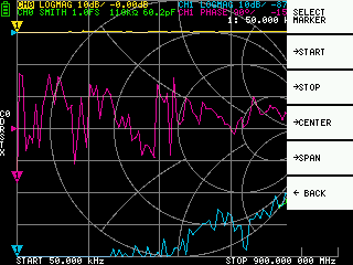
You can set the frequency range from the marker as follows.

MARKER →START Set the frequency of the active marker to the start frequency
MARKER →STOP Sets the frequency of the active marker to the stop frequency
MARKER →CENTER Sets the active marker frequency to the center frequency. The span is adjusted to maintain the current range as much as possible.
MARKER →SPAN Set the two displayed markers, including the active marker, to the span. Nothing happens if only one marker is displayed.

Setting the measurement range

There are three types of measurement range settings.

Set the start frequency and stop frequency
Set center frequency and span
Zero span

Set the start frequency and stop frequency

Select and set STIMULUS START and STIMULUS STOP , respectively.

Set center frequency and span

Select and set STIMULUS CENTER and STIMULUS SPAN respectively.

Zero span

Zero span is a mode in which one frequency is transmitted continuously without performing a frequency sweep.

Select and set STIMULUS CW FREQ .

Stop measurement temporarily

Selecting STIMULUS PAUSE SWEEP temporarily stops measurement.

Recall calibration and settings

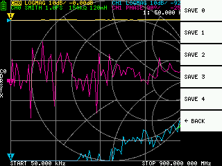
Up to five calibration data can be stored. Immediately after NanoVNA starts, it loads the data with number 0.

Calibration data is data that contains the following information:

Frequency setting range
Error correction at each measurement point
Trace setting status
Marker setting status
Domain mode settings
Setting the wavelength shortening rate
electrical delay

CAL current settings can be saved by selecting CAL SAVE SAVE n .

You can reset the current calibration data by selecting CAL RESET . To re-calibrate, you need to RESET .

CAL CORRECTION indicates whether error correction is currently being performed. You can select this to temporarily stop error correction.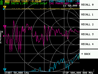

RECALL saved settings by selecting RECALL RECALL n .

Device settings

Below CONFIG , general settings of the device can be made.

Touch panel calibration and test

CONFIG you select CONFIG TOUCH CAL , you can calibrate the touch panel. If there is a large difference between the actual tap position and the recognized tap position, this can be solved by doing so. After performing TOUCH CAL , perform TOUCH TEST to confirm that the settings are correct, and save the settings using SAVE .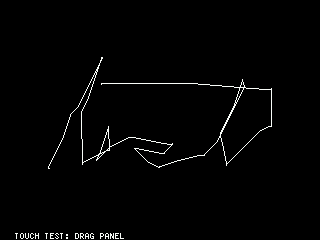

CONFIG you select CONFIG TOUCH TEST , you can test the touch panel. While tapping the touch panel, a line is drawn. It returns to the original state when released from the touch panel.

Saving device settings

Select CONFIG SAVE to save general device settings. General device settings are data that includes the following information:

Touch panel calibration information
Grid color
Trace color
Calibration data number loaded by default

There is currently no way to make settings other than touch panel calibration information.

Show version

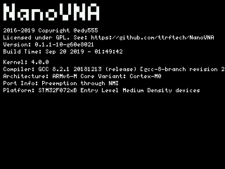
Select CONFIG VERSION to display device version information.

Firmware update

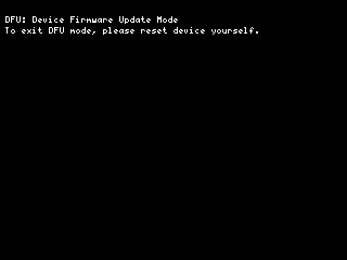
Select CONFIG →DFU RESET AND ENTER DFU to reset the device and enter DFU (Device Firmware Update) mode. In this mode, the firmware can be updated via USB.

How to update the firmware

How to get the firmware

ttrftech version firmware

Original firmware. It is version controlled and is frequently developed.

GitHub releases has a somewhat stable release version of the firmware.

CircleCI has all the firmware for every commit. Use this if you want to try the latest features or check for bugs.

hugen79 version firmware

Google Drive

Google Drive has the latest firmware.

Build yourself

You can easily clone the github repository and build it yourself.

How to write firmware

There are various ways to write, but here we explain using dfu-util . dfu-util is a cross-platform tool, and binaries are provided on Windows, so you can use it just by downloading it.

Writing with dfu-util (Ubuntu)

There is dfu-util in the standard package repository.

 sudo apt-get install dfu-util dfu-util --version

Start the device in DFU mode. Enter the DFU mode in one of the following ways.

Turn on the power while jumping the BOOT0 pin on the PCB. (Remove the jumper after turning on the power.) The screen turns white, but it is normal.
CONFIG →DFU Select →DFU RESET AND ENTER DFU

Execute the following command. build / ch.bin describes the path to the downloaded firmware file .bin.

 dfu-util -d 0483:df11 -a 0 -s 0x08000000:leave -D build/ch.bin

Writing using dfu-util (macOS)

It is recommended to install using homebrew .

Install the brew command.

 ruby -e "$(curl -fsSL https://raw.githubusercontent.com/Homebrew/install/master/install)" 

Install the dfu-util command.

 brew install dfu-util

Check that the dfu-util command can be started normally.

 dfu-util --version

Start the device in DFU mode. Enter the DFU mode in one of the following ways.

Turn on the power while jumping the BOOT0 pin on the PCB. (Remove the jumper after turning on the power.) The screen turns white, but it is normal.
CONFIG →DFU Select →DFU RESET AND ENTER DFU

Execute the following command. build / ch.bin describes the path to the downloaded firmware file .bin.

 dfu-util -d 0483:df11 -a 0 -s 0x08000000:leave -D build/ch.bin

Writing using dfu-util (Windows 10)

In Windows, when a NanoVNA in DFU mode is connected, the device driver is installed automatically. However, this device driver cannot use dfu-util. Here, the driver is exchanged using Zadig .

Start the device in DFU mode. Enter the DFU mode in one of the following ways.

Turn on the power while jumping the BOOT0 pin on the PCB. (Remove the jumper after turning on the power.) The screen turns white, but it is normal.
CONFIG →DFU Select →DFU RESET AND ENTER DFU

Start Zadig with the NanoVNA in DFU mode connected, and use WinUSB as a driver for STM32 BOOTLOADER as shown below.

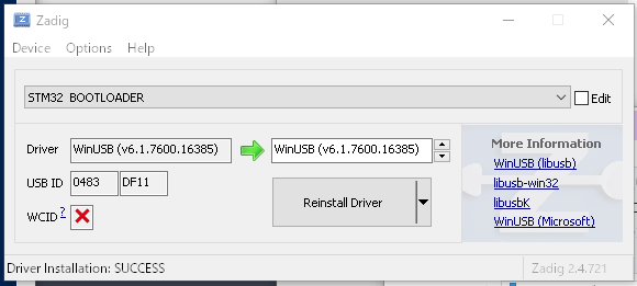
* If you want to restore the driver, search for the applicable device from "Universal Serial Bus Controller" in "Device Manager" and execute "Uninstall Device". Unplug the USB connector and plug it in again, the driver will be installed automatically.

Next, place dfu-util. Download dfu-util-0.9-win64.zip from releases and extract it. Here, it is assumed that it is expanded to C: \ dfu-util as an example (anywhere is fine).

Right-click on the start menu and select Windows PowerShell. The shell screen opens.

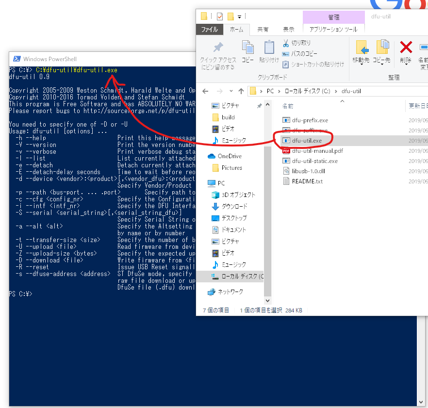
Drag and drop dfu-util.exe from Explorer to PowerShell and the path will be inserted automatically. You can display the version of dfu-util by starting with --version as shown below.

 C:\dfu-util\dfu-util.exe --version

Similarly, you can enter the path of the firmware file by dragging and dropping it from Explorer to PowerShell.

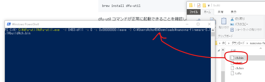
Execute the following command. build / ch.bin describes the path to the downloaded firmware file .bin.

 C:\dfu-util\dfu-util.exe -d 0483:df11 -a 0 -s 0x08000000:leave -D build\ch.bin

How to write firmware (Windows GUI)

For those who are unfamiliar with CUI, some complicated steps are required, but the writing method using the DfuSE Demo tool provided by ST is introduced for reference only.

Download STSW-STM32080 from the ST site .

DFU File Manager: Tool to create .dfu files from .bin or .hex
DfuSe Demo: Tool to write .dfu files to device

is included.

Convert file format with DFU File Manager.

First, launch DFU File Manager.

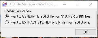
Select I want to GENERATE a DFU file from S19, HEX or BIN files .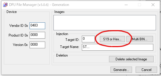

Click the S19 or Hex... button. ch.hex firmware ch.hex file, such as ch.hex .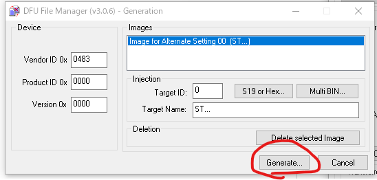

Click the Generate... button and create a .dfu file with a suitable name.

Write firmware with DfuSe Demo

First, boot the device in DFU mode. Enter the DFU mode in one of the following ways.

Turn on the power while jumping the BOOT0 pin on the PCB. (Remove the jumper after turning on the power.) The screen turns white, but it is normal.
CONFIG →DFU Select →DFU RESET AND ENTER DFU

Start DfuSe Demo. Make sure there is STM Device in DFU Mode Available DFU Devices and click Choose...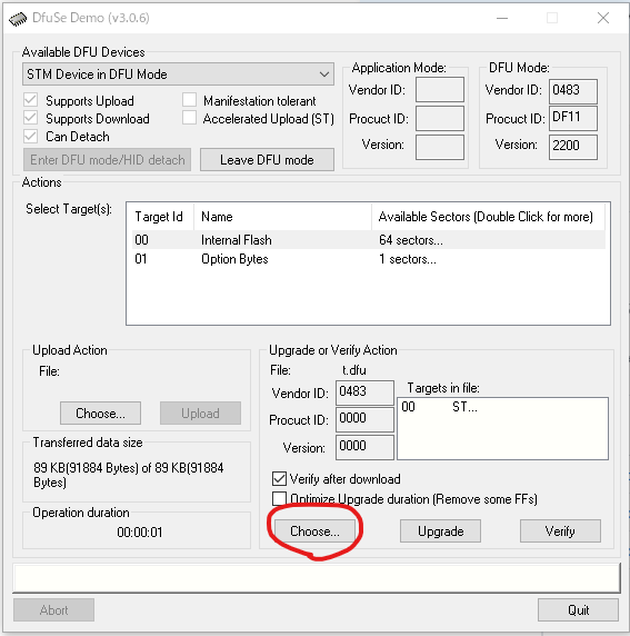

Select the .dfu file you just saved.

Click the Upgrade button.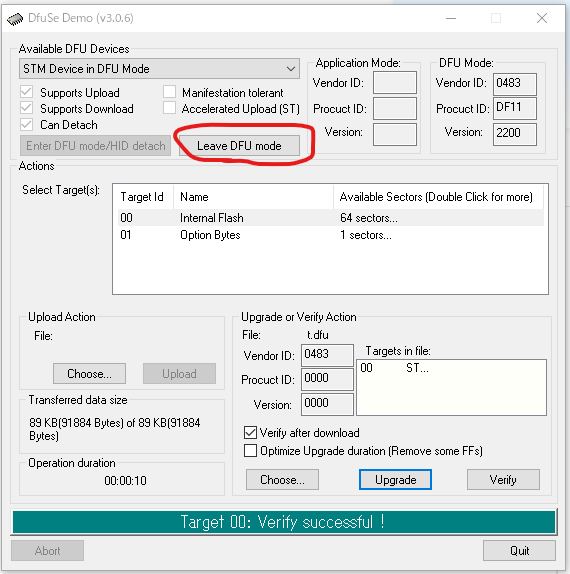

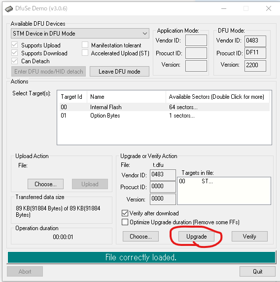
This screen will be displayed when writing is completed. Click the Leave DFU mode button to exit DFU mode. The device will reset and boot with the new firmware.

Firmware Development Guide

The following items need to be developed for NanoVNA firmware.

Git
gcc-arm-none-eabi
make

If you already have these, you can build the firmware with make .

 git clone git@github.com:ttrftech/NanoVNA.git cd NanoVNA git submodule update --init --recursive make 

Build with Docker

With docker you can build without hassle. docker is a free cross-platform container utility. It can be used to quickly recreate a particular environment (in this case, a build environment).

Just run the following command after installing docker .

 docker run -it --rm -v $(PWD):/work edy555/arm-embedded:8.2 make

On-chip debugging with Visual Studio Code

Visual Studio Code (VSCode) is a multi-platform code editor provided by Microsoft free of charge. By installing Cortex-Debug Extension, on-chip debugging can be performed by GUI.

The platform-dependent part is omitted, but the following is required in addition to the above.

openocd
VSCode
Cortex-Debug

Cortex-Debug is searched from Extensions of VSCode and installed.

tasks.json

First, define a "task" to make the entire NanoVNA on VSCode.

 { 
     "tasks" :   [ 
         { 
             "type" :   "shell" , 
             "label" :   "build" , 
             "command" :   "make" , 
             "args" :   [ 
             ], 
             "options" :   { 
                 "cwd" :   "${workspaceRoot}" 
             } 
         } 
     ], 
     "version" :   "2.0.0" 
 } 
 

Now you can make it as a task on VSCode.

launch.json

Next, define how it will be launched during Debug. Set as described in Cortex-Debug.

The following is the setting when using ST-Link. If you use J-Link, replace interface/stlink.cfg with interface/jlink.cfg .

 { 
     "version" :   "0.2.0" , 
     "configurations" :   [ 
         { 
             "type" :   "cortex-debug" , 
             "servertype" :   "openocd" , 
             "request" :   "launch" , 
             "name" :   "OpenOCD-Debug" , 
             "executable" :   "build/ch.elf" , 
             "configFiles" :   [ 
                 "interface/stlink.cfg" , 
                 "target/stm32f0x.cfg" 
             ], 
             "svdFile" :   "./STM32F0x8.svd" , 
             "cwd" :   "${workspaceRoot}" , 
             "preLaunchTask" :   "build" , 
         } 
     ] 
 } 
 

svdFile file specified in svdFile can be downloaded from the ST site . svdFile is no problem in operation even if svdFile is not specified.

Start debugging

When Start Debugging ( F5 ) is performed, OpenOCD is automatically started and firmware is transferred after build by make. When the transfer is completed, a break occurs at the reset handler.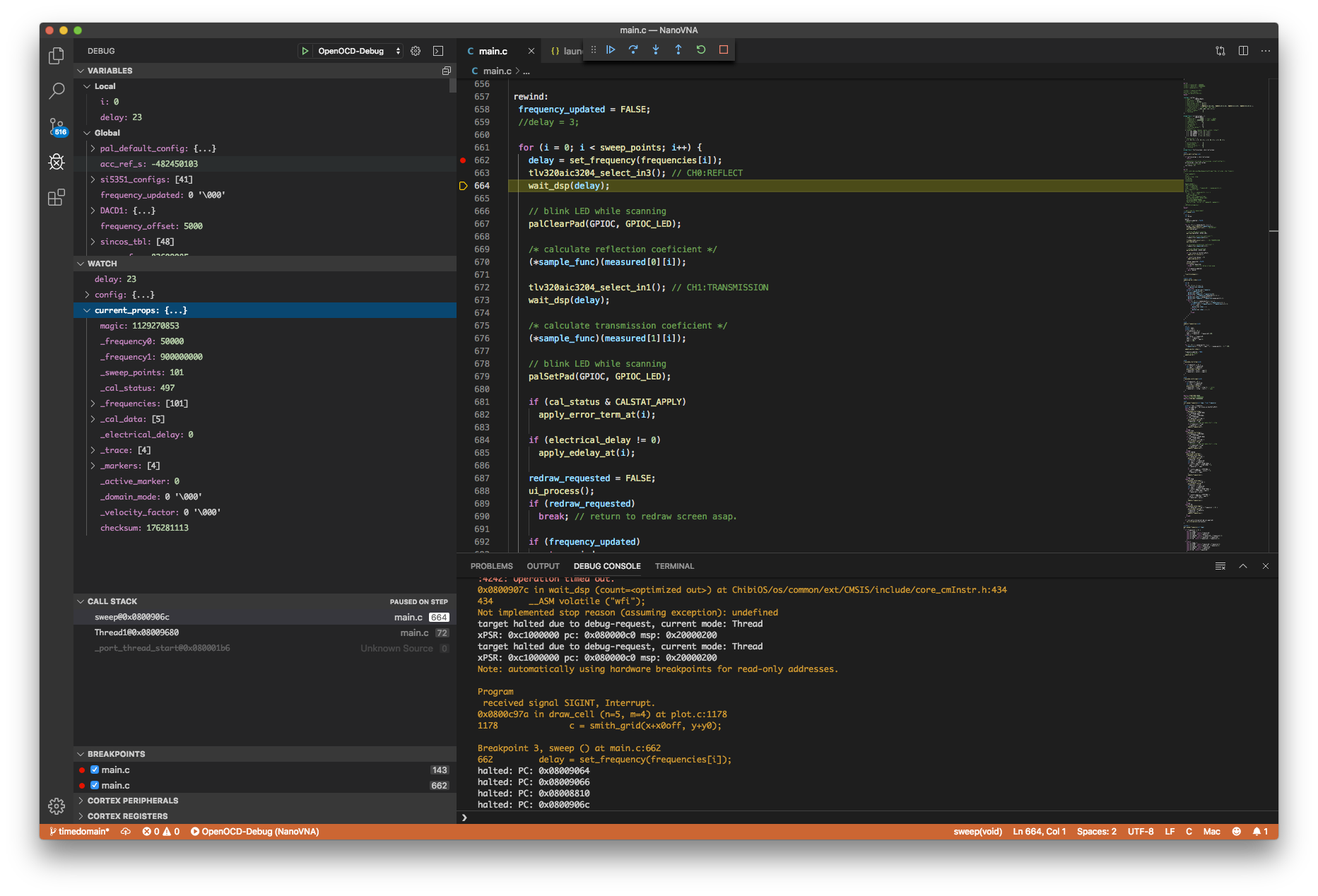

svdFile is specified, the registers of the defined MCU are displayed on the debug screen.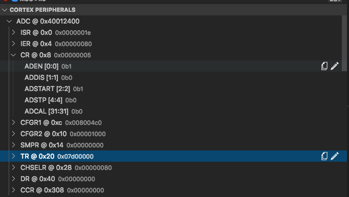

Example of use

Adjusting the bandpass filter

TODO

Adjusting the antenna

Here is an example of using NanoVNA as an antenna analyzer.

There are two important points in adjusting the antenna:

Whether the antenna is in tune and resonance (that is, the reactance is close to 0 at the target frequency)
Is the SWR of the antenna low (sufficient matching)

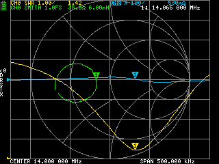
Trace settings

Since only CH0 is used for antenna adjustment, calibrate all items except THRU and ISOLN .

Set the trace settings as follows.

Trace 0: CH0 SWR
Trace 1: CH0 REACTANCE
Trace 2: CH0 SMITH
Trace 3: OFF

Set the desired frequency for tuning the antenna to CENTER and set SPAN appropriately.

Look for frequencies where trace 1 showing reactance is close to zero. Since the frequency is the tuning point, if it is off, adjust the antenna so that the tuning point comes to the target frequency.

If the tuning point is at the desired frequency, check that Trace 0, which is displaying SWR, is displaying a sufficiently low (close to 1) SWR. If it does not show enough (less than 2) SWR, it will be matched using a Smith chart. In this case, matching may be performed using an antenna tuner directly below the antenna.

If the SWR drops, you are tuned to the desired frequency and you are finished tuning the low SWR antenna.

Check cable

You can simulate TDR by using the low-pass mode in the time domain. By using TDR, it is possible to detect transmission line defects.

TODO

Common mode filter measurement

TODO

*************************************************

NanoVNA User Guide

Introduction

What is NanoVNA

What you need to work

NanoVNA Basics

Oscillation frequency of NanoVNA

First thing to do

input method

How to read the screen

Main screen

1. START 2. STOP frequency

3. Markers

4. Calibration status

5. Reference position

6. Marker status

7. Trace status

8. Battery status

Main screen 2

9. CENTER frequency 10. Span

Menu screen

11. Menu

Keypad screen

12. Numeric keys

13. Back key

14. Unit key

15. Input field

Start measurement

Basic measurement sequence

Calibration method

function

Trace display

Trace format

Trace channel

marker

Time domain operation

Time domain bandpass

Time domain low pass impulse

Time domain low pass step

Step response example

Time domain window

Setting the Velocity Factor in the time domain

Set frequency from marker

Setting the measurement range

Set the start frequency and stop frequency

Set center frequency and span

Zero span

Stop measurement temporarily

Recall calibration and settings

Device settings

Touch panel calibration and test

Saving device settings

Show version

Firmware update

How to update the firmware

How to get the firmware

ttrftech version firmware

hugen79 version firmware

Build yourself

How to write firmware

Writing with dfu-util (Ubuntu)

Writing using dfu-util (macOS)

Writing using dfu-util (Windows 10)

How to write firmware (Windows GUI)

Convert file format with DFU File Manager.

Write firmware with DfuSe Demo

Firmware Development Guide

Build with Docker

On-chip debugging with Visual Studio Code

tasks.json

launch.json

Start debugging

Example of use

Adjusting the bandpass filter

Adjusting the antenna

Trace settings

Check cable

Common mode filter measurement

Pesquisar este blog